Installation, operation and technical reference for the PathGridData Generator
(CPSQDSIM) – a site-specific quasi-deterministic channel model simulator developed
at the Radio Signal Processing Laboratory, Niigata University.
As wireless technology evolves, new communication systems must keep pace with the demands of
autonomous driving, drones, IoT and Beyond 5G. The frequency band below 6 GHz is becoming
increasingly congested, so improving spectrum utilisation and increasing signal bandwidth are
necessary to raise transmission speed and data volume. This has led to renewed interest in
millimeter-wave communication, which uses the 30–300 GHz band and can enable gigabit
transmission rates. As the number of millimeter-wave devices grows, systems must be developed
quickly and designed to respond to a wide variety of scenarios, which in turn demands accurate
evaluation of the propagation channel.
Because of its short wavelength, the millimeter-wave band has quasi-optical properties and strong
rectilinearity, and it can carry large amounts of information – but free-space propagation loss
and attenuation due to transmission, diffraction and scattering are significant drawbacks. Where a
line-of-sight (LoS) path exists, specular reflection components are the primary propagation paths
alongside the LoS. Geometric optical methods (ray tracing) can accurately predict the main
propagation paths in a simple environment, and reproducing an environment-specific model more
accurately improves prediction accuracy. In complex environments, however, prediction becomes
increasingly challenging as processing time grows prohibitive. In addition, the short wavelength
means that surface irregularities of reflective materials play a significant role in causing diffuse
scattering, which is difficult to simulate accurately.
In this situation a quasi-deterministic (Q-D) model is used to represent environment-specific
propagation paths. It combines deterministic components – LoS and one- to two-bounce reflections
obtained by simple ray tracing – with probabilistic components such as random scatterers and
diffuse scattering clusters associated with specular reflection, modelled through statistical
distributions. A pure Q-D model is limited in how accurately it represents an individual
environment because it relies on statistical distributions derived from measurements in typical
scenarios. A hybrid channel model combining deterministic and probabilistic components is
therefore necessary, and developing one requires a large volume of channel data and a clear
understanding of the propagation characteristics.
To gather environment-specific channel data in an urban macrocell setting, a channel sounder
capable of measuring bi-angular propagation channels in both the 24 and 60 GHz bands was used,
allowing simultaneous measurement in both bands. Elementary waves were extracted from the
collected data with an ultra-high-resolution channel estimation algorithm and classified into
clusters by similar delay and angle. Combining the 24 GHz and power-compensated 60 GHz
multipaths made it possible to cluster both frequencies at the same time, identify the propagation
path of each cluster, and obtain statistical characteristics of power difference and relative delay
for clusters common to both frequencies.
2. Technical Specification
2.1 Overview of the propagation model layers
The hybrid quasi-deterministic propagation model calculates the dominant propagation paths using
simple ray tracing for direct waves and large structures, while using probabilistic calculations for
small objects such as trees and signboards. The inputs are the rays generated by ray tracing and
the statistical parameters (LSPs, SSPs) used to generate propagation paths probabilistically. LSP
values matching the actual environment can also be derived by feeding 3D map data into a
machine-learning model.
The output, PathGridData, contains path power, delay and departure/arrival angles. It is
calculated and stored for each grid point at a fixed spatial interval, and is then handed to the
wireless emulator so that the channel response at an arbitrary point can be obtained. The
generation flow applies probabilistic compensation to the deterministic clusters computed by ray
tracing, based on the cluster delay–power characteristics obtained by measurement, and
introduces site-specific LSPs/SSPs to obtain more accurate propagation characteristics for the
target environment.
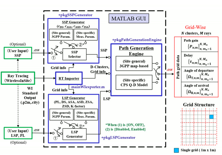
Figure 2.1 – CPSQDSIM framework. Ray-tracing output and the user parameter
inputs are fed into the SSP Generator, LSP Generator and Path Generation Engine to produce
grid-wise PathGridData. The Path Generation Engine supports both the site-general 3GPP map-based
model and the site-specific NU (CPS QD) model. In the current GUI the SSP parameter table is a
required input and the LSP/PL file is optional; the internal handling is otherwise unchanged
(see §6.2 a).
2.2 Evaluation, measurement and model parameter extraction
The propagation channel was examined in the vicinity of Yokohama World Porters, a six-storey
commercial complex in Kanagawa Prefecture. The base station (BS) was fixed and the mobile station
(MS) was moved to 25 locations (#001–#025) along an L-shaped path around the outer perimeter of
the facility. Measurements used two frequencies simultaneously and lasted approximately five
minutes at each location.
Item
Value
Site
Yokohama World Porters, Kanagawa Prefecture, Japan
Frequencies
24 GHz and 60 GHz (simultaneous)
MS positions
25 locations (#001–#025) along an L-shaped route
MS spacing
≈1 m for #009–#023; ≈10 m for the remaining positions
Tx–Rx distance
24–109 m
Antenna heights
Tx (BS) 3 m, Rx (MS) 1.5 m
Link conditions
Downlink (BS: Tx, MS: Rx), line-of-sight
Scenario
Millimeter-wave urban microcell (UMi) – BS on a streetlight, MS a mobile terminal
Duration
≈5 minutes per location
2.3 Post-processing
2.3.1 Extraction of multipath components
After noise removal is applied to the measured DDADPS data, the sub-grid CLEAN algorithm extracts
the multipath components (MPCs). The algorithm measures a power image (replica) of an MPC,
calculated from the continuous horizontal-plane antenna pattern and the autocorrelation function
of the sounding signal (a sinc function for rectangular spectra such as multitone). It then applies
successive interference cancellation (SIC) to perform maximum-likelihood estimation, subtracting
power sequentially in order of magnitude. This yields finer-resolution MPC estimates that are not
influenced by the horizontal-plane antenna pattern or the signal bandwidth. An angular resolution
of 0.1° and a delay resolution of 0.01 ns were achieved.
2.3.2 Clustering
The extracted MPCs are clustered into groups by angle and delay. The composite datasets of MPCs
obtained at each frequency are used for clustering. To account for the increased propagation loss
caused by the frequency difference, the power of each 60 GHz MPC is increased by
20 log10(58.32 / 24.15) = 7.66 dB. After clustering, the MPCs are separated back
into their respective frequency datasets and the 60 GHz powers are restored to their original
values. This identifies clusters common to both frequencies as well as clusters unique to one of
them. Clustering uses the K-PowerMeans algorithm; the number of clusters K is determined
manually by visual inspection so that the results retain physical meaning.
2.4 Channel model parameters
The channel parameters consist of LSPs and SSPs. LSPs represent the spatio-temporal power spread
of the clusters, while SSPs represent the spatio-temporal power spread of the MPCs within a
cluster.
Large-scale parameters (LSPs)
Computed over the clusters of a link: delay spread (DS), azimuth spread of departure (ASD)
and of arrival (ASA), zenith spread of departure (ZSD) and of arrival (ZSA), and the Ricean
K-factor. DS is the power-weighted RMS spread of the cluster delays; the angular spreads use
the circular (complex exponential) definition.
Small-scale parameters (SSPs)
The intra-cluster delay spread (cDS) and intra-cluster angular spreads (cASD / cASA),
derived from the individual MPCs inside each cluster using the same power-weighted
definitions applied within a cluster.
Recipe parameters (RPs)
Parameters of the exponential-decay model used to calibrate deterministic cluster power,
refining the 3GPP map-based model where detailed building orientation, dimension and
dielectric data are not available.
Exponential decay model for recipe parameters
Obtaining detailed data on the orientation, dimensions and dielectric properties of every building
object in the evaluation area is essential for a truly accurate depiction of deterministic clusters,
but this is impractical in complex urban settings with a large separation between transmission and
reception points. An exponential decay model is therefore used to calibrate deterministic cluster
power. For the power delay characteristics of NLoS clusters it takes the form:
P(τ) = P0 + 10 log10 exp(−τ / τ0) + SF
where P0 is the initial path gain, τ0 the delay decay factor, and
SF the standard deviation of the cluster shadowing variation, which is treated as a zero-mean
Gaussian shadowing term.
2.5 Power compensation for NLoS deterministic clusters
The deterministic NLoS cluster power is obtained from the decay model for each BS–MS link.
Compensation is applied using the z-score of the power deviation from the model, in three steps:
The difference between the delay-decay line of the cluster power and the deterministic
(ray-traced) cluster power is calculated for each cluster.
The z-score of that difference is calculated using its mean and standard deviation over the
applicable clusters.
The compensated cluster power is obtained by adding the scaled shadowing term back onto the
decay model, giving the realistic cluster power used in PathGridData generation.
Note
The full set of equations, including the exact index ranges applied to LoS and NLoS links and the
delay-attenuation characteristics measured at 24 and 60 GHz, is given in the CPSQDSIM project
report and in the IEEE TVT paper listed in
Chapter 11.
3. Installation
CPSQDSIM is distributed as a standalone Windows desktop application: a GUI for generating channel
data, exploring maps and multipath components, and exporting the data as CSV files. The
application and the site data are distributed separately.
Install the application
Download the Windows installer and run it; follow the setup wizard.
Install the matching MATLAB Runtime when prompted. The application will not
start without the runtime version it was compiled against.
Install the site data
Download the site-data package for the frequency you intend to simulate – the
matching map and ray-tracing dataset for the study area.
Extract it into a writable folder that is separate from the application
installation folder.
Writable output folder
Do not place generated projects inside the installation folder. Choose a separate, writable
location for both the extracted site data and the simulation output directory.
3.1 Demo run
The installer sets up a demo dataset in the input fields automatically, so the installation can be
verified before any site data is prepared. The demo consists of a small sample of receiver grids
selected near the base station; pressing Run generates the outputs for them. The
information bar states that file saving is off, and that the input files can be replaced with your
own site data when you are ready.
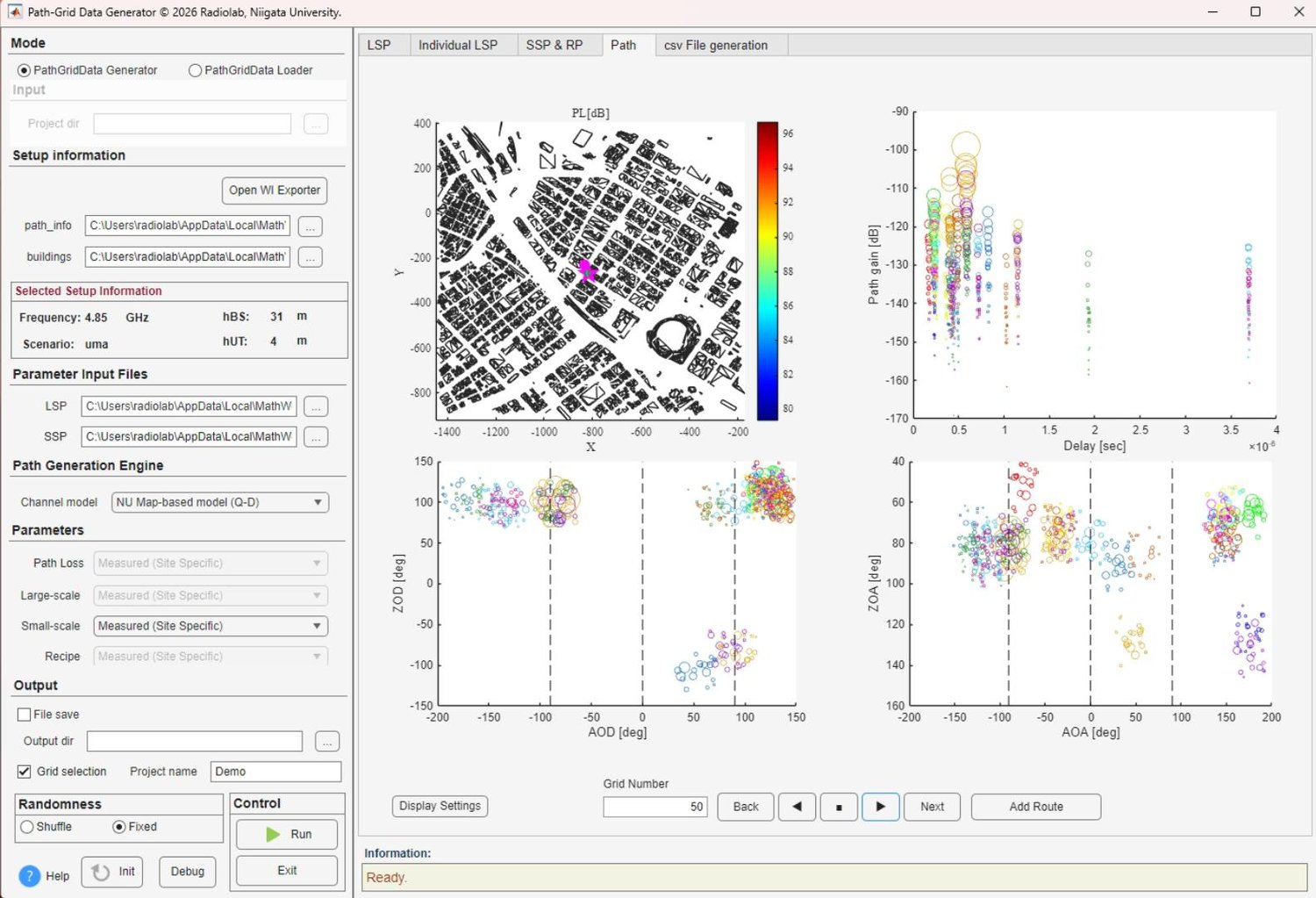
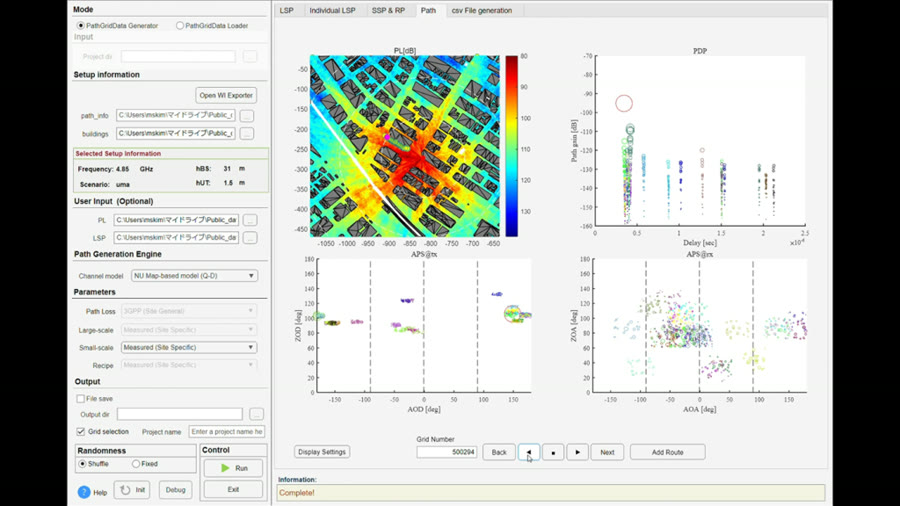
Figure 3.1 – Demo run, Path tab: the path-loss map with the demo receiver
route near the transmitter, and the corresponding delay, AoD/ZoD and AoA/ZoA plots.
Demo defaults
The demo is configured with the project name Demo, Grid selection
enabled, Fixed randomness and File save off – a receiver route
close to the transmitter, at 4.85 GHz, UMa, hBS 31 m, hUT 4 m.
Enable File save and set an output directory when you want the results written to
disk.
4. Quick Start
The steps below are the shortest route from a fresh installation to an exported dataset. Each step
links to the detailed reference later in this manual.
#
Step
What to do
1
Install
Run the installer, install the MATLAB Runtime, extract the site-data package to a
writable folder. §3
2
Try the demo run
The installer pre-loads a demo dataset. Press Run to confirm the
installation works before preparing your own site data. §3.1
3
Prepare ray-tracing input
If path_info.mat and buildings.mat are already available, use them
directly. Otherwise generate them from the Wireless InSite output with the WI Exporter
sub-app. §5
4
Choose PathGridData Generator
Select path_info and buildings, then check the displayed frequency,
scenario and Tx/Rx heights. §6.2
5
Set model and inputs
Choose the path generation engine and the parameter sources; add matching user PL or LSP
CSV files when available. §6.2
6
Select receiver grids
Enable Grid selection. For a route, pick points and press
connect; for an area, choose a shape, press Draw and close the
region of interest. Check the preview and apply it to the main app.
§6.2
7
Save and run
Enable File save, choose an output folder and project name, and press
Run. Choose Fixed randomness to repeat a run with the same setup.
Wait for the completion message. §6.2
8
Read the results
Inspect the LSP, Individual LSP, SSP & RP and Path tabs.
§7
9
Export
Open csv File generation and press File Generate to write the
emulator CSV files into the project folder. §8
5. WI Exporter – preparing the ray-tracing input
In the main application window, the ray-tracing (Wireless InSite) input is supplied by two files:
path_info.mat and buildings.mat. A sub-application, opened with
open WI Exporter, extracts the required information from the Wireless InSite output and
generates those two files.
When is the WI Exporter needed?
If path_info.mat and buildings.mat already exist they can be used directly in
the main window. The sub-app must be used the first time, whenever a different WI project is used,
or whenever the WI files have changed.
The exporter requires six inputs before it can produce the .mat files:
1. Project Name
The name assigned to the project when the Wireless InSite software was run. It can be identified
from the folder name created when the WI project completed – for example Tx38.
2. p2m folder location
The p2m_folder is created under the main project folder when the WI project completes.
It contains many files, of which only a few are needed for import. Confirm that the required
*.paths and *.pl files with the .p2m extension are present; their
exact names vary with the project name and the order in which Wireless InSite was executed.
3. City file location
The city file is generated when the Wireless InSite project completes. Ensure that a
building.city file exists in the folder; if the file has a different name, rename the
*.city file to building.city and select that folder.
4. ID range
The p2m folder may contain several files with the same extension distinguished by a
number in the file name – for example xxxxx.r007.p2m and xxxxx.r008.p2m.
All *.paths and *.pl files with the .p2m extension are required, so
in that example the ID range must be specified as 7 to 8.
5. Scenario, frequency, hBS and hUT
Specify the scenario, the frequency and the BS and UT heights exactly as they were set during the
Wireless InSite run. The frequency must be given in GHz.
6. Output file location
Specify the folder in which the generated .mat files will be stored for further
processing.
7. Export
If all the information above is correct, the sub-app generates building.mat and
path_info.mat in the specified output folder, together with the final map view of the
exported area.
6. Main Window – Left Panel
All user input for a run is provided through the left panel of the main application window: the
environment, the scenario and the generation options are set there before generation starts. The
application accepts site-specific measured path loss and large-scale parameter values as user
input, which gives the most accurate result for the target environment.
PathGridData Loader – load previously generated PathGridData together with the
related files.
6.2 PathGridData Generator
Upload the two input files – path_info.mat and buildings.mat. Once they are
uploaded, the setup information (frequency, scenario, BS and UT heights) is displayed for
confirmation.
a) Parameter input files – LSP and SSP
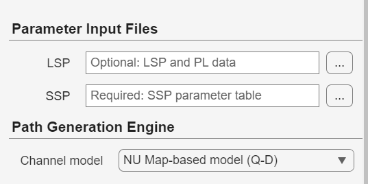
The Parameter Input Files section takes two CSV inputs:
Figure 6.1 – The Parameter Input Files section: the LSP box is optional and
carries both LSP and PL data, while the SSP parameter table is required.
Box
Status
Contents
LSP
Optional – LSP and PL data
Site-specific measured path loss and large-scale parameter values for each grid, in a
single CSV file. Path loss and LSPs share this one input; there is no separate PL box.
If it is left empty, PL and LSPs are generated from the parameter sources selected in
(c).
SSP
Required – SSP parameter table
The small-scale parameter table used by the SSP generator. This input is mandatory;
the site-data package on Zenodo supplies LSP_SSP_Table.csv for this
purpose.
Column order is strict
Each LSP input must follow the order
Grid ID, PL, DS, ASD, ASA, ZSD, ZSA, K. A different order will be interpreted
incorrectly and will produce an incorrect result.
b) Path generation engine
Engine
Description
NU map-based model (Q-D)
Follows the exponential decay model described in §2.4, with
recipe-parameter calibration of the deterministic cluster power.
3GPP map-based model (Q-D)
Follows the channel modelling approach of 3GPP TR 38.901 version 16.1.0 Release 16.
c) Parameters
Select the parameter sources used to generate the PathGridData:
Path loss – if a site-specific PL CSV file was already uploaded, the PL selection
box stays inactive. If no PL file was provided, choose a path-loss option so that PL values are
generated for each grid following the 3GPP recommendation.
LSP – if no user LSP CSV file is provided, LSPs can be generated either from the
measured (site-specific) statistical parameter values, or from the 3GPP site-general
recommended values.
SSP – as with the LSPs, small-scale parameters can follow either the site-specific
statistical parameter values or the 3GPP site-general values.
d) Recipe parameter
The recipe parameter implements the NU exponential-decay model. It is assigned automatically when
the NU path generation engine is selected. If the 3GPP engine is chosen it becomes inactive,
because the 3GPP model has no recipe-like statistical parameter.
e) Output directory and project name
Check File Save to save the output files, then specify the directory in which they will
be written. The Project Name text box creates a corresponding folder under the output
directory. If it is left blank, the default folder name is untitled – or
untitled_01 and so on when several projects already exist – and the output files are
saved there.
f) Grid selection
This opens a new window showing the entire map with the buildings, so that a particular route or
area can be selected and PathGridData generated only for the chosen grids. A route can be created
in two ways:
Select more than one grid on the map and click connect to join the selected grids
into a route.
Specify a CSV file containing the grid IDs that make up the route and press
Apply.
For an area rather than a route, choose a shape, press Draw and close the region of
interest. The selection is shown in the preview area on the right-hand side; check it, then apply
it to the main application.
Run time
Running all grids in the study area takes substantially longer than running a small selected grid
area. Start with a route or a limited region of interest, and reserve a full-area run for when the
settings have been confirmed.
g) Randomness
This panel controls how the statistical values are drawn. Select Fixed when the same
values must be reproduced across several runs, for example for testing; use Shuffle to
draw new random values on each execution.
h) Control panel
Run starts the generation of the PathGridData and Exit closes the
application window. Wait for the completion message before moving on.
6.3 PathGridData Loader
The loader is used to view channel behaviour quickly for each grid in the form of path loss, LSPs
and SSPs, when the folder and files generated by CPSQDSIM already exist. Select the
Project dir in which the previously generated files are stored and press
Run; the information bar reports when loading has completed. In the
SSP & RP tab, use the load button to read the summary.
Note
When the PathGridData Loader option is selected, the other options in the left panel become
inactive.
7. Main Window – Right Panel
The right panel displays the generated results. Four tabs are available.
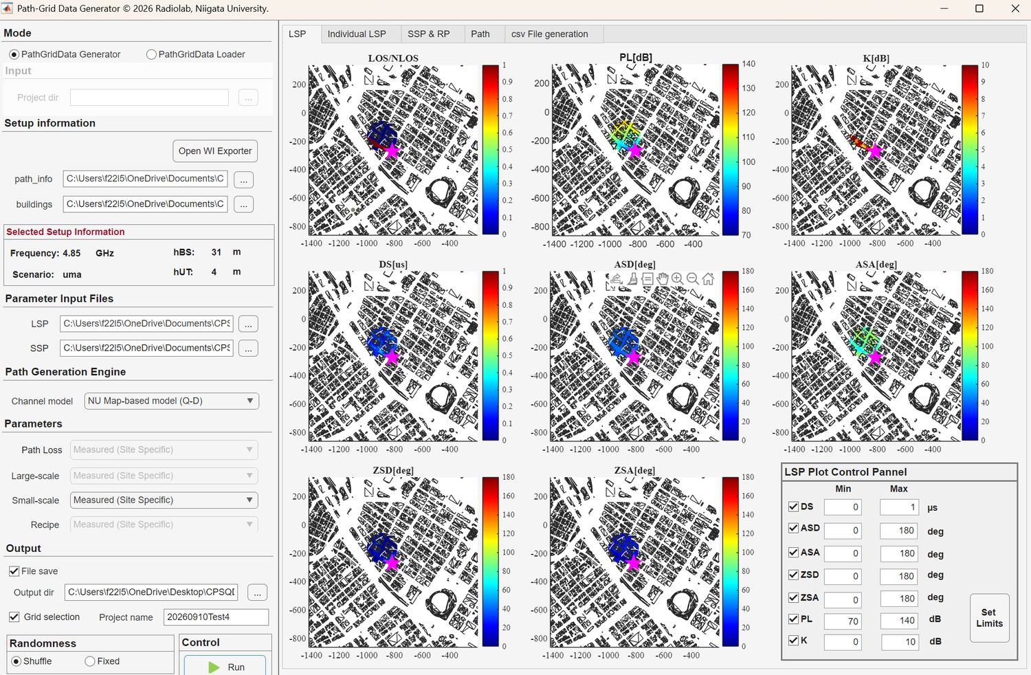
Figure 7.1 – Main window, LSP tab: LoS/NLoS, PL, K, DS, ASD, ASA, ZSD and
ZSA maps for the selected grids, with the LSP Plot Control Panel setting the colour limits.
The left panel shows the current Parameter Input Files layout.
Figure 7.2 – Path view showing the delay–angle power spectrum (PDP, APS)
for individual grid points.
LSP tab
Displays the generated LoS/NLoS condition, path loss and LSPs in separate plots. A control box in
the lower-right corner of the window sets the minimum and maximum range of the LSP values shown on
the map, so that the colour limits can be matched across parameters.
Individual LSP tab
Displays one selected LSP on the map over a larger area. Use the select button below the plot to
choose the desired LSP or PL from the drop-down box.
SSP & RP tab
Presents the stochastic small-scale parameter values used to create the SSP values for each grid,
together with the general information for the run. Recipe parameter values are also displayed if
the NU map-based model was used, or if the recipe was chosen in the left panel during parameter
selection. Otherwise the tab is left empty.
Path tab
If a route was selected in the grid-selection window during generation, this tab shows the current
properties in four plot areas – path loss, PDP, angular power spectrum at the Tx (APS@Tx) and at
the Rx (APS@Rx) – at each Rx point as the MS moves along the selected route. The playback buttons
below the plots (play, next, pause, previous and back) move the current MS position forwards and
backwards along the route. On the map (PL plot) the red circle indicates the current Rx location
and the yellow circles represent the route. The Display Setting button sets the minimum
and maximum display values.
8. CSV Export for the CPS Emulator
The CSV file generation window creates the files corresponding to the PathGridData that the
emulator requires. Specify the location of the project folder that has already been created, then
click File Generate: the necessary .mat files are loaded, converted to CSV
and saved in the same project folder. Depending on the size of the .mat files this may
take a few minutes. Three files are produced.
File
Contents
dcdl_condition_…MHz_Rx…m.csv
Frequency and transmitter position
dcdl_area_data_…MHz.csv
Receiver coordinates
dcdl_path_…MHz_Rx…m.csv
Path delays, angles and gains
Condition file – e.g. dcdl_condition_4850MHz_Rx4m.csv
condition_id
frequency
tx_point_x
tx_point_y
tx_point_z
1
28350
-818.418
-270.731
32.89
Area data file – e.g. dcdl_area_data_4850MHz.csv
condition_id
rx_id
rx_point_x
rx_point_y
rx_point_z
1
1
-1414
-864
4
1
2
-1413
-864
4
1
3
-1412
-864
4
1
4
-1411
-864
4
Path file – e.g. dcdl_path_28350MHz_Rx4m.csv
condition_id
rx_id
path_id
path_delay
path_aod
path_zod
path_aoa
path_zoa
path_distance
path_gain
1
13966
1
6.40E-07
-132.7
98.7
47.3
81.3
10
-124.7
1
13966
2
6.40E-07
-130.8
99.1
49.7
82.5
10
-143.7
1
13966
3
6.40E-07
-138.3
99.9
14.3
89.2
10
-168.0
1
13966
4
6.40E-07
-150.4
98.7
30.1
86.1
10
-158.5
Angles are given in degrees, delay in seconds and path gain in dB.
9. Simulation Results & Verification
The generated PathGridData was verified against measured data by comparing the CDFs of the delay
and angular spreads over all grid points in the evaluation area. The simulation environment used
for the verification was:
Setting
Value
Scenario
UMa (urban macrocell)
hBS
31 m
hUT
4 m
LSP
DS, ASA, ASD, ZSA, ZSD – user input (KDDI)
K-factor
3GPP TR 38.901 Table 7.5-6, UMa
SSP
3GPP TR 38.901 Table 7.5-6, UMa
PL
User input (KDDI)
Frequencies verified
28350 MHz, 4850 MHz, 2462 MHz, 922 MHz
For each frequency, the CDFs of the delay and angle spreads obtained with the PathGridData
Generator following the site-specific NU map-based model were compared with the measured data,
taking all grid points in the entire area.
The CDFs indicate that the results closely match the measured data at all four frequencies, which
supports the validity and accuracy of the simulation model. Comparing the CDF plots against both
the existing 3GPP map-based model and the measured data shows that the NU model aligns more
closely with the measurements. Some discrepancies remain: the CDFs of ASA, particularly at the
sub-6 GHz frequencies, show a significant gap between the measured data and the simulated
result, and further analysis is needed to improve how the model reflects site-specific
characteristics.
10. Summary & Conclusion
Item
Description
Project title
R&D for the realization of a high-precision radio wave emulator in cyberspace
(JPJ000254)
Main objective (Group A)
To model a site-specific channel model (propagation layer) following the NU map-based
model, producing PathGridData that contains detailed information at each grid position
(Rx point) – delay, power and angle of departure/arrival – for use in channel
emulators and for network performance analysis and optimisation.
Development objective
To design a customised channel model and simulation software that can rapidly and
effectively produce PathGridData for the channel emulator (managed by a separate team),
enabling comprehensive testing of channel behaviour ahead of field testing or real-world
implementation.
Specific objective
To enhance the accuracy of predicting channel characteristics in the mmWave and sub-6 GHz
bands, reflecting site-specific radio-wave characteristics more accurately than existing
channel models.
(a) The R-layer, providing the ray-tracing files for each frequency and scenario;
(b) actual measured data for those frequencies and scenarios.
Outputs
PathGridData for each frequency and scenario as .mat files and corresponding
.csv files – eight output sets in total, for four frequencies at two MS
heights (4 m and 9 m).
11. Publications
IEEE TVT 2025
H. Tsukada, N. Suzuki, B. Bag, R. Takahashi and M. Kim,
"Millimeter-Wave Urban Cellular Channel Characterization and Recipe for High-Precision
Site-Specific Channel Simulation," IEEE Trans. Veh. Technol., vol. 74, no. 3,
pp. 3598–3612, Mar. 2025.
10.1109/TVT.2024.3492719
EuCAP 2023
M. Kim, N. Suzuki, H. Tsukada and R. Takahashi,
"Frequency Dependence of Millimeter-Wave Urban Macrocell Multipath Cluster Channels,"
in Proc. European Conference on Antennas and Propagation (EuCAP), Florence, Italy,
Mar. 2023.
Dataset 2026
M. Kim and I. Calist, "CPSQDSIM: Site-Specific Channel Model Simulator," Ver. 1.0, Zenodo, 2026.
10.5281/zenodo.22644137
12. Bibliography
"Study on channel model for frequencies from 0.5 to 100 GHz (3GPP TR 38.901 version 16.1.0
Release 16)," Nov. 2020.
[Online]. Available:
etsi.org
S. Jaeckel et al., "QuaDRiGa – Quasi-deterministic radio channel generator, user manual and
documentation," Wireless Commun. Netw. Dept., Fraunhofer Heinrich Hertz Institute, Berlin,
Germany, Rep. V2.0.0, Aug. 2017.
K. Haneda, J. Järveläinen, A. Karttunen, M. Kyrö and J. Putkonen,
"A Statistical Spatio-Temporal Radio Channel Model for Large Indoor Environments at 60 and
70 GHz," IEEE Trans. Antennas Propag., vol. 63, no. 6, pp. 2694–2704, 2015.
About this manual
This manual consolidates the CPSQDSIM final project report (Radio Lab, Niigata University,
December 2024) and the CPSQDSIM operation manual for the standalone Windows build (September 2026).
For questions regarding the simulator or collaboration inquiries, contact
Prof. Minseok Kim –
mskim@eng.niigata-u.ac.jp.